Methods of Contour Surveying

Methods of Contour Surveying

There are two methods of contour surveying:

[1]. Direct method

[2]. Indirect method

Direct Method of Contouring

   It consists in finding vertical and horizontal controls of the points which lie on the selected contour line.

   For vertical control levelling instrument is commonly used. A level is set on a commanding position in the area after taking fly levels from the nearby bench mark. The plane of collimation/height of instrument is found and the required staff reading for a contour line is calculated.

  The instrument man asks staff man to move up and down in the area till the required staff reading is found. A surveyor establishes the horizontal control of that point using his instruments.

After that instrument man directs the staff man to another point where the same staff reading can be found. It is followed by establishing horizontal control.

Thus, several points are established on a contour line on one or two contour lines and suitably noted down. Plane table survey is ideally suited for this work.

After required points are established from the instrument setting, the instrument is shifted to another point to cover more area. The level and survey instrument need not be shifted at the same time. It is better if both are nearby to communicate easily.

For getting speed in levelling some times hand level and Abney levels are also used. This method is slow, tedious but accurate. It is suitable for small areas.

Indirect Method of Contouring

In this method, levels are taken at some selected points and their levels are reduced. Thus in this method horizontal control is established first and then the levels of those points found.

After locating the points on the plan, reduced levels are marked and contour lines are interpolated between the selected points.

For selecting points any of the following methods can be used:

[1]. Method of squares

[2]. Method of cross-section

[3]. Radial line method

Method of Squares

In this method area is divided into a number of squares and all grid points are marked (Fig. Con. 10).

  

                        

Commonly used size of square varies from 5 m × 5 m to 20 m × 20 m. Levels of all grid points are established by levelling. Then grid square is plotted on the drawing sheet. Reduced levels of grid points marked and contour lines are drawn by interpolation (Fig. Con. 10).

Method of Cross-Section

In this method cross-sectional points are taken at regular interval. By levelling the reduced level of all those points are established. The points are marked on the drawing sheets, their reduced levels (RL) are marked and contour lines interpolated.

  

  Fig. Con. 11 shows a typical planning of this work. The spacing of cross-section depends upon the nature of the ground, scale of the map and the contour interval required. It varies from 20 m to 100 m. Closer intervals are required if ground level varies abruptly.

   The cross- sectional line need not be always be at right angles to the main line. This method is ideally suited for road and railway projects.

 

Radial Line Method

(Fig. Con. 12). In this method several radial lines are taken from a point in the area. The direction of each line is noted. On these lines at selected distances points are marked and levels determined. This method is ideally suited for hilly areas. In this survey theodolite with tacheometry facility is commonly used.

               

   For interpolating contour points between the two points any one of the following method may be used:

(a) Estimation

(b) Arithmetic calculation

(c) Mechanical or graphical method.

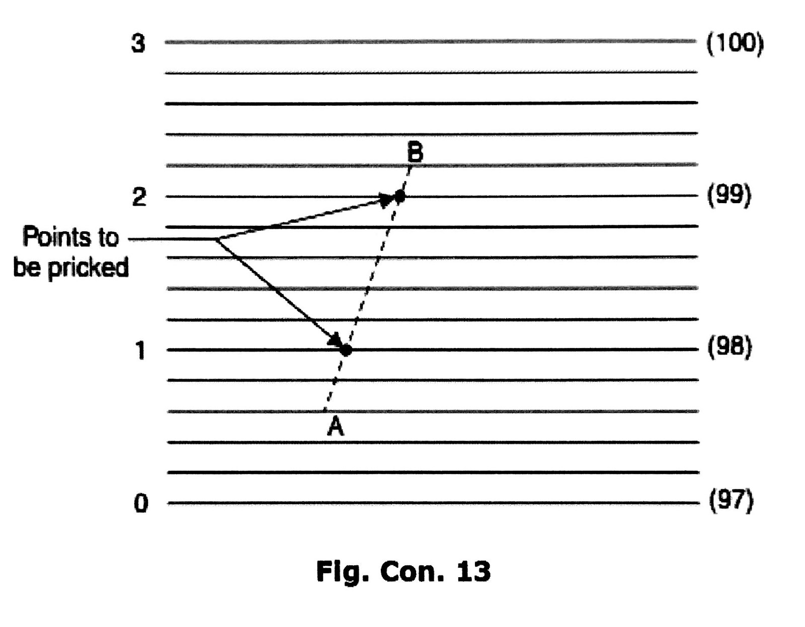
Mechanical or graphical method of interpolation consist in linearly interpolating contour points using tracing sheet:

   On a tracing sheet several parallel lines are drawn at regular interval. Every 10th or 5th line is made darker for easy counting. If RL of A is 97.4 and that of B is 99.2 m. Assume the bottom most dark line represents 97 m RL and every parallel line is at 0.2 m intervals. Then hold the second parallel line on A.

   Rotate the tracing sheet so that 100.2 the parallel line passes through point B. Then the intersection of dark lines on AB represents the points on 98 m and 99 m contours (Fig. Con. 13).

 

   Similarly the contour points along any line connecting two neighbouring points may be obtained and the points pricked. This method maintains the accuracy of arithmetic calculations at the same time it is fast.

                             

Drawing Contours

   After locating contour points smooth contour lines are drawn connecting corresponding points on a contour line. French curves may be used for drawing smooth lines. A surveyor should not lose the sight of the characteristic feature on the ground. Every fifth contour line is made thicker for easy readability. On every contour line its elevation is written. If the map size is large, it is written at the ends also.

Contour Gradient
   Gradient represents the ascending or descending slope of the terrain between two consecutive contour lines. The slope or gradient is usually stated in the format 1 in S, where 1 represents the vertical component of the slope and S its corresponding horizontal component measured in the same unit.

   The gradient between two consecutive contour lines can also be expressed in terms of tanθ as follows:
tanθ = Contour Interval (CI) /Horizontal Equivalent (HE) … both     measured in the same unit.

Location of Contour Gradient

   To locate a rising gradient of 1 in 100 from the station P, a level is set up at a commanding position and back sight is taken at P. Let the back sight reading be 1.255 m. The staff reading at any point X on the contour gradient can be calculated from its distance from P (Fig. Con. 14). For the distance XP of 20 m, the required staff reading would be

        1.255 - (20/100) = 1.055

   To locate the point X on the ground, the staff man holds the 20 m-mark of the tape, keeping the zero-mark at P, and moves till the staff reading of 1.055 m is obtained. Likewise, the staff readings for other points at known distance from P, are calculated, and the points are located. If the point Q is on the contour of 105 m, its distance from P would be 500 m in this case. The instruments such as Indian clinometer, theodolite and Ghat tracer may also be used for tracing the contour gradient on the ground.

CONTOURING

CONTOURING

Contour line: A Contour line is an imaginary outline of the terrain obtained by joining its points of equal elevation. In our example of the cone, each circle is a contour line joining points of same level.

Contour interval: A contour interval in surveying is the vertical distance or the difference in the elevation between the two contour lines in a topographical map. Usually there are different contour intervals for the different maps.

Horizontal equivalent: The horizontal distance between two points on two consecutive contour lines for a given slope is known as horizontal equivalent.

  

USES OF CONTOUR MAPS

   Contour maps are extremely useful for various civil engineering works as explained below:

[1]. Preliminary selection of project sites: Characteristics of contour lines give considerable information about nature of ground. Sitting in the office studying contour lines, a civil engineer decides various possible sites for his project.

[2]. Drawing of sections: From contour plan, it is possible to study profile of the ground along any line, which is normally required for earthwork calculation along a formation ground.

[3]. Determination of intervisibility: If intervisibility of any two points is to be checked, using contour, profile of the ground along the line joining those two points can be drawn. Then the line joining those two points is drawn. If the ground portion is above this portion, the two stations are not intervisible.

 [4]. Location of routes: The routes of railway, road, canal or sewer lines can be decided with the help of contour maps. After deciding the gradient of the route, it can be set on the map as explained.

[5]. Determining catchment Area; The area on which fallen rainwater drains into river at a particular point is called catchment area of the river at that point. This area can be determined from contour plans. The catchment area is also known as drainage area. First the line that separates the catchment basin from the rest of area is drawn. This is called watershed time. It normally follows ridge line. Then the area within watershed line is measured. This area is extremely useful in studying flood level and quantity of water flow in the river.

[6]. Calculation of reservoir capacity: The submerged area and the capacity of a proposed reservoir by building bund or dam can be found by using contour maps. After determining the height of the dam its full reservoir level is known. Then area between any two contour lines and the dam line is measured by using plan meter to find the reservoir capacity.

CHARACTERISTICS OF CONTOUR

The principal characteristics of contour lines which help in plotting or reading a contour map are as follows:

[1]. Contour lines must close, not necessarily in the limits of the plan.

[2]. The horizontal distance between any two contour lines indicates the amount of slope and varies inversely on the amount of slope.

[3]. Widely spaced contour indicates flat surface (Fig. Con.2).

[4]. Closely spaced contour indicates steep slope ground (Fig. Con.2).

 [5]. Equally spaced contour indicates uniform slope.

[6]. Irregular contours indicate uneven surface (Fig. Con.3).

[7]. Approximately concentric closed contours with decreasing values towards centre indicate a pond (Fig. Con.4).

[8]. Approximately concentric closed contours with increasing values towards centre indicate hills (Fig. Con.5).

[9]. Contour lines with U-shape with convexity towards lower ground indicate ridge (Fig. Con.6.a).

[10]. Contour lines with V-shaped with convexity towards higher ground indicate valley (Fig. Con.6.b).

[11]. Contour lines generally do not meet or intersect each other. If contour lines are meeting in some portion, it shows existence of a vertical cliff (Fig. Con. 7).

       

[12]. Contours of different elevations cannot cross each other. If contour lines cross each other, it shows existence of overhanging cliffs or a cave (Fig. Con. 8).

    

[13]. The steepest slope of terrain at any point on a contour is represented along the normal of the contour at that point.

[14]. Contours do not pass through permanent structures such as buildings (Fig. Con. 9).

 

[15]. A contour line must close itself but need not be necessarily within the limits of the map.

(Next post on “METHODS OF CONTOUR”)

RECIPROCAL LEVELLING

RECIPROCAL LEVELLING

   We have found by the principle of equalizing backsight and foresight distances that if the level is placed exactly midway between two points and staff reading are taken to determine the difference of level, then the errors (due to inclined of collimation line, curvature and refraction) are automatically eliminated. But in the case of a river or valley, it is not possible to set up the level midway between the two points on opposite banks. In such case the method of reciprocal levelling is adopted, which involves reciprocal observation both banks of the river or valley.

   In reciprocal leveling, the level is set up on the both banks of the river or valley and two sets of staff readings are taken by holding the staff on both banks. In this case, it is found that the errors are completely eliminated and true difference of level is equal to the mean of the true apparent differences of level.

Procedure  

[1]. Suppose A and B are two points on the opposite banks of a river. The level is set up near A and after proper temporary adjustment, staff readings are taken at A and B. Suppose the readings are a₁ and b₁ (Fig. – L.23.a).

[2]. The level is shifted and set up very near B and after proper adjustment, staff reading are taken at A and B. suppose the readings are a₂ and b₂ (Fig. – L.23.b).

Let     h = true difference of level between A and B

          e = combined error due curvature, refraction and collimation (The error may be positive or negative, here we assume positive)

In the first case,

Correct staff reading at A = a₁         (as the level very near A)

Correct staff reading at B = b₁ - e

True difference between A and B,

           h = a₁ – (b₁ – e)    (fall from B to A)   ……. (1)

In the second case,

Correct staff reading at B = b₂         (as the level very near B)

Correct staff reading at A = a₂ - e

True difference of level,

           h = (a₂ –e) - b₂            …….……. (2)

From (1) and (2), 

           2h = a₁ – (b₁ – e) + (a₂ – e) - b₂

                = a₁ – b₁ + e + a₂ – e - b₂

              h = [(a₁ – b₁)+(a₂ – b₂)]/2

It may be observed that the error is eliminated and that the true difference is equal to the mean of two apparent differences of level between A and B.

(Next post on “METHODS OF CALCULATION OF REDUCE LEVEL”)

PRINCIPLE OF EQUALISING BACKSIGHT AND FORESIGHT DISTANCES

PRINCIPLE OF EQUALISING BACKSIGHT AND FORESIGHT DISTANCES

   In levelling, the line of collimation should be horizontal when the staff readings are taken. Again the fundamental relation is that the line of collimation should be exactly parallel to the axis of the bubble. So, when the bubble is at the centre of its run, the line of collimation is just horizontal. But sometimes the permanent adjustment of level may be disturbed and the line of collimation may not be parallel to the axis of the bubble. In such case, due to the inclination of the line of collimation, cross in levelling are lickly to occur. But it is found that if the backsight and foresight distances are kept equal, then the error due to the inclination of the collimation line is automatically eliminated.

Case I – When the line of collimation inclined upwards Let A and B be two points whose true difference of level is required. The level is set up at O, exactly midway between A and B (Fig. – L.16).

Let θ = angle of inclination of collimation line.

   Aa = true reading

  Aa₁ = observed staff reading on A

Error = Aa₁ - Aa = aa₁ = D tanθ

So true reading Aa = Aa₁ - aa₁ = Aa₁ - D tanθ     ………..(1)

Similarly, Bb = true reading

Bb₁ = observed staff reading on B

Error = Bb₁ - Bb = bb₁ = D tanθ

So true reading Bb = Bb₁ - bb₁ = Bb₁ - D tanθ    ………….(2)

From (1) and (2),

True difference of level between A and B = Aa – Bb

                                               = Aa₁ - D tanθ - Bb₁ + D tanθ

                                               = Aa₁ - Bb₁

Thus, this is seen that the error due to inclination of the collimation line is completely eliminated and the apparent difference is equal to the true difference.

Case II – When the line of collimation inclined downwards The staff readings on A and B are taken after setting the level at O. Suppose the readings are a₂ and b₂ (Fig. – L.17).

Here,   Aa = true staff reading

  Aa₂ = observed staff reading on A

Error = Aa - Aa₂ = aa₂ = D tanθ

So true reading Aa = Aa₂ + aa₂ = Aa₂ + D tanθ     ………..(1)

Similarly, Bb = true reading

Bb₂ = observed staff reading on B

Error = Bb - Bb₂ = bb₂ = D tanθ

So true reading Bb = Bb₂ + bb₂ = Bb₂ + D tanθ    ………….(2)

From (1) and (2),

True difference of level between A and B = Aa – Bb

                                                     = Aa₂ + D tanθ - Bb₂ - D tanθ

                                                     = Aa₂ - Bb₂

Thus, this is seen that the error due to inclination of the collimation line is completely eliminated and the apparent difference is equal to the true difference.

So, always remember that the level should be placed exactly midway between backsight and foresight in order to eliminate any error.

CORRECTION TO BE APPLIED

(1). Curvature correction: For long sights, the curvature of the earth effect staff readings. The line of sight is horizontal, but the level line is curved and parallel to the mean spheroidal surface of the earth (Fig. – L.18).   

   The vertical distance between the line of sight and level line at a particular place is called the curvature correction. Due to curvature, objects appear lower than they really are.

Curvature correction always subtractive (i.e. negative) 

Let   AB = D = horizontal distance in kilometers.

       BD = Cc = curvature correction

       DC = AC = R = radius of earth

       DD’ = diameter, considered as 12742 km

From right angle triangle ABC (Fig. – L.19).

  

     BC² = AC² + AB²

     (R + Cc) ² = R² + D²

or  R² + 2RCc + Cc² = R² + D²

or  2R X Cc = D²     (Cc² is neglected as it is very small in comparison to the

                                 diameter of the earth)

Curvature correction   Cc = D²/2R

Cc = (D² x 1000)/12742 = 0.0785D² m   (negative)

Hence,   True staff reading = observed staff reading – curvature correction.

(2). Refraction correction: Rays of light are refracted when they pass through layers of air of varying density. So, when long sights are taken, the line of sight refracted towards the surface of the earth in a curved path. The radius of this curve seven times that of the earth under normal atmospheric conditions. Due to the effect of refraction, objects appear higher than they really are. But the effect of curvature varies with the atmospheric conditions.

However, on an average, the refraction correction is taken one-seventh of the curvature correction.

               Cr = 1/7 x D²/2R

Refraction correction, Cr = 1/7 x 0.0785D² = 0.0112D² m (positive)

Refraction correction is always additive (i.e. positive)

True reading = observed staff reading + refraction correction

(3). Combined correction: The combined effect of curvature and refraction is as follows:

Combined correction = curvature correction + refraction correction

                               = -0.0785D² + 0.0112D²

                               = -0.0673D² m

So, combined correction always subtractive (i.e. negative)

True reading = observed staff reading - combined correction

Combined correction may also be expressed as

                          D²/2R – 1/7 x D²/2R = 6/7 x D²/2R   (negative)

(4). Visible horizon distance

Let    AB = D = visible horizon distance in kilometers (Fig. – L.20).

Considering curvature and refraction corrections,

                       h = 0.0673D²

                       D = √(h/0.0673)

(5). Dip of horizon

AB = D = tangent of earth at A

BD = horizontal line perpendicular to OB

θ = dip of horizon

The angle between the horizontal line and the tangent line is known as the dip of the horizon. It is equal to the subtended by the arc AC at the centre of the earth (Fig. – L.21).

Dip θ = arc AC/radius of earth     in radians

θ = D/R, in radians  (Taking AC approx, equal to AB)

 

Hear, D and R must be expressed in the same unit.

(6). Sensitiveness of the bubble: The term sensitiveness in the context of a bubble means the effect caused by the deviation of the bubble per division of the graduation of the bubble tube.

   Sensitiveness is expressed in term of the radius of the curvature of the upper surface of the tube or by an angle through which the axis is tilted for the deflection of one division of the graduation.

Determining sensitiveness: consider Fig. L.22. Suppose the level was set up at O at a distance D from the staff at P. The staff reading is taken with the bubble at extreme right end (i.e. at E). Say it is PA. Another staff reading taken with the bubble at the extreme left end (i.e. at E₁). Let it is be PB  

Let,   D = distance between level and staff

        S = intercept between the upper and lower sights,

        n = number of divisions through the bubble is reflected,

        R = radius of curvature of the tube,

        θ = angle subtended by arc EE₁, and

        d = length of the division of the graduation, expressed in the same unit

              as D and S.

Movement of centre of bubble = EE₁ = nd

Triangle OEE₁ and ACB are similar.

Here,           Rθ = arc EE₁

or                θ = EE₁/R = nd/R   …….(1)   (as arc EE₁ = chord EE₁)

Again           EE₁/R = S/D   (height of triangle OEE₁ may be considered as R)

or                 nd/R = S/D      ……………. (2)

From (1) and (2),    

                   θ = nd/R = S/D   …………(3)

Therefore,      R = (nd x D)/S

Let                θ’ = angular value for one division in radians

                     θ’ = θ/n = S/D x 1/n radians

                    

                     θ’ = S/(D x n) x 206265 secs. (1 radian = 206265 secs.)

(Next post on “RECIPROCAL LEVELLING”)